Idealized Fracture Test Problem for Numerical Homogenization Methods
Contents:
|
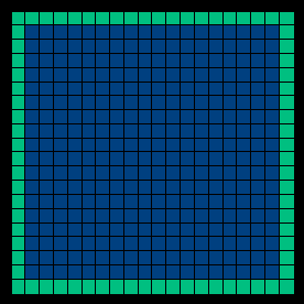
Map Image For 5% Fracture
|
Map Image For 10% Fracture
|
|

|
Problem Description
This page describes the idealized fracture periodic test problem for
homogenization tests. This test problem is about the simplest idealization of a
fracture network that one can imagine. The idealized fractures generated in this
way is similar to the pattern defined in the
symmetric cell test problem,
based on a 4 by 4 grid. However, the symmetric fracture pattern involves a thin
border region of higher permeability around a square lower permeability region
as shown below. The idealized fracture is useful in double porosity models and
can be used to study homogenization methods tailored to fracture problems.
Problem/Data Links:
The following is a list of raw data sets that can be downloaded and used as
input for your own homogenization codes for testing, input to reservoir
simulators and other applications. These maps can also be downloaded and used
as input for the JHomogenizer application.
- 5 percent fracture width:
- 10 percent fracture width:
Homogenization Results:
The following documents the results for various homogenization methods applied
to the idealized fracture. The results are for coefficient ratios of 10 to 1 and
100 to 1 for the fracture region relative to the interior portions of the
pattern. The values used are given at the top of the table along with the output
tensor values in the last column. These results are used to generate some of the
data sets used to compare simulation results given below.
The two fracture patterns documented on this page include a fracture region that
is only 5% and 10% of the region along the coordinate directions. Examples are
shown above on a 20 by 20 grid.
5 Percent Fracture Width Results
|
Coefficient Ratio:
|
Homogenization Method:
|
Homogenization Tensor:
|
|
10:1
|
|
|
|
|
Arithmetic Average:
|
| 2.7099 |
0.0000 |
0.0000 |
| 0.0000 |
2.7099 |
0.0000 |
| 0.0000 |
0.0000 |
2.7099 |
|
|
|
Geometric Average:
|
| 1.5488 |
0.0000 |
0.0000 |
| 0.0000 |
1.5488 |
0.0000 |
| 0.0000 |
0.0000 |
1.5488 |
|
|
|
Harmonic Average:
|
| 1.2063 |
0.0000 |
0.0000 |
| 0.0000 |
1.2063 |
0.0000 |
| 0.0000 |
0.0000 |
1.2063 |
|
|
|
HomCode Average:
|
| 2.0211 |
0.0000 |
0.0000 |
| 0.0000 |
2.0211 |
0.0000 |
| 0.0000 |
0.0000 |
2.7100 |
|
|
|
Linear Boundary Condition Average:
|
| 2.0309 |
0.0000 |
0.0000 |
| 0.0000 |
2.0309 |
0.0000 |
| 0.0000 |
0.0000 |
2.7100 |
|
|
|
Fractured Media Tensor Average:
|
Not Applicable
|
|
|
Linear Boundary Condition Wavelet Average:
|
Not Applicable
|
|
|
Periodic Wavelet Average:
|
Not Applicable
|
|
100:1
|
|
|
|
|
Arithmetic Average:
|
| 19.810 |
0.0000 |
0.0000 |
| 0.0000 |
19.810 |
0.0000 |
| 0.0000 |
0.0000 |
19.810 |
|
|
|
Geometric Average:
|
| 2.3988 |
0.0000 |
0.0000 |
| 0.0000 |
2.3988 |
0.0000 |
| 0.0000 |
0.0000 |
2.3988 |
|
|
|
Harmonic Average:
|
| 1.2317 |
0.0000 |
0.0000 |
| 0.0000 |
1.2317 |
0.0000 |
| 0.0000 |
0.0000 |
1.2317 |
|
|
|
HomCode Average:
|
| 11.3591 |
-0.457861E-05 |
0.0000 |
| -0.457861E-05 |
11.3591 |
0.0000 |
| 0.0000 |
0.0000 |
19.810 |
|
|
|
Linear Boundary Condition Average:
|
| 11.432 |
0.0000 |
0.0000 |
| 0.0000 |
11.432 |
0.0000 |
| 0.0000 |
0.0000 |
19.810 |
|
|
|
Fractured Media Tensor Average:
|
Not Applicable
|
|
|
Periodic Wavelet Average:
|
Not Applicable
|
|
|
Linear Boundary Condition Wavelet Average:
|
Not Applicable
|
10 Percent Fracture Width Results
|
Coefficient Ratio:
|
Homogenization Method:
|
Homogenization Tensor:
|
|
10:1
|
|
|
|
|
Arithmetic Average:
|
| 4.2310 |
0.0000 |
0.0000 |
| 0.0000 |
4.2310 |
0.0000 |
| 0.0000 |
0.0000 |
4.2310 |
|
|
|
Geometric Average:
|
| 2.2909 |
0.0000 |
0.0000 |
| 0.0000 |
2.2909 |
0.0000 |
| 0.0000 |
0.0000 |
2.2909 |
|
|
|
Harmonic Average:
|
| 1.4793 |
0.0000 |
0.0000 |
| 0.0000 |
1.4793 |
0.0000 |
| 0.0000 |
0.0000 |
1.4793 |
|
|
|
HomCode Average:
|
| 3.0889 |
0.0000 |
0.0000 |
| 0.0000 |
3.0889 |
0.0000 |
| 0.0000 |
0.0000 |
4.2400 |
|
|
|
Linear Boundary Condition Average:
|
| 3.1125 |
0.0000 |
0.0000 |
| 0.0000 |
3.1125 |
0.0000 |
| 0.0000 |
0.0000 |
4.2400 |
|
|
|
Fractured Media Tensor Average:
|
Not Applicable
|
|
|
Linear Boundary Condition Wavelet Average:
|
Not Applicable
|
|
|
Periodic Wavelet Average:
|
Not Applicable
|
|
100:1
|
|
|
|
|
Arithmetic Average:
|
| 36.640 |
0.0000 |
0.0000 |
| 0.0000 |
36.640 |
0.0000 |
| 0.0000 |
0.0000 |
36.640 |
|
|
|
Geometric Average:
|
| 5.2481 |
0.0000 |
0.0000 |
| 0.0000 |
5.2481 |
0.0000 |
| 0.0000 |
0.0000 |
5.2481 |
|
|
|
Harmonic Average:
|
| 1.5538 |
0.0000 |
0.0000 |
| 0.0000 |
1.5538 |
0.0000 |
| 0.0000 |
0.0000 |
1.5538 |
|
|
|
HomCode Average:
|
| 22.300 |
-0.145664E-05 |
0.0000 |
| -0.145664E-05 |
22.300 |
0.0000 |
| 0.0000 |
0.0000 |
36.640 |
|
|
|
Linear Boundary Condition Average:
|
| 22.502 |
0.0000 |
0.0000 |
| 0.0000 |
22.502 |
0.0000 |
| 0.0000 |
0.0000 |
36.640 |
|
|
|
Fractured Media Tensor Average:
|
Not Applicable
|
|
|
Periodic Wavelet Average:
|
Not Applicable
|
|
|
Linear Boundary Condition Wavelet Average:
|
Not Applicable
|
Simulation Results:
The following graphics show results for simulations performed on a heterogeneous
maps and the homogenized maps that result from applying various methods of
averaging. The heterogeneous map used in the generation of the flow simulations
looks like the map below. The simulation results shown below were obtained using
maps generated by the JHomogenizer tool. The graphics below were generated using
the JHomogenizer tool.
Example 1: 4x4 Periodic Fracture Pattern - 80x80 blocks:
To show how using homogenization results effect the solution of the elliptic
problem the following case is considered. The idealized fracture heterogeneous
used in the simulations is shown below.

In this example the idealized fracture is repeated in two dimensions a total of
4 times in each of the coordinate directions. This means that there are a total
of 80 small blocks blocks in the region on which the simulations are performed.
The set of figures below show the saturation from the solution of a simple two
phase flow equation. The fluxes are determined from a solution of an elliptic
equation for the head/pressure variable. The use of the lowest order mixed
finite element method gives the approximations of the fluxes that are used as
input into a simple upwind method for approximately solving the flow equation.
Solutions below are shown for the heterogeneous data set and data sets that
result from the homogenization methods. As you can see, the results for the
homogenized regions are not distinguishable and completely wash out the
structure of the fracture pattern. This suggests that a blind approach using
homogenization will produces less than acceptable results. To see more on this
problem you can look at the
Idealized Fracture benchmark
problem.
Heterogeneous Solution for 10:1 Coefficient Ratio
|
Elliptic Solution
|
Flux Approximation
|
Flow Approximation (2500 Steps)
|

|

|

|
Heterogeneous Solution for 100:1 Coefficient Ratio
|
Elliptic Solution
|
Flux Approximation
|
Flow Approximation (2500 Steps)
|

|

|

|
Homogenized Results
Arithmetic Average Simulations
|
Elliptic Solution
|
Flux Approximation
|
Flow Approximation (2500 Steps)
|

|

|

|
Geometric Average Simulations
|
Elliptic Solution
|
Flux Approximation
|
Flow Approximation (2500 Steps)
|

|

|

|
HomCode Average Simulations
|
Elliptic Solution
|
Flux Approximation
|
Flow Approximation (2500 Steps)
|

|

|

|
Linear Boundary Condition Average Simulations
|
Elliptic Solution
|
Flux Approximation
|
Flow Approximation (2500 Steps)
|

|

|

|
Harmonic Average Simulations
|
Elliptic Solution
|
Flux Approximation
|
Flow Approximation (2500 Steps)
|

|

|

|
Steps to use JHomogenizer to create and work with the idealized fracture map:
To create the results included on these pages you can use the JHomogenizer tool.
The instructions for creating homogenization results are in the following how to
file.