The Exact Solution of the Gambler's Ruin Problem

Now let's return to the difference equation we have above. The solution method is virtually the same as that in the two examples in the previous section. First assume a solution form

$$s_c(a) = z^a$$

for some unknown base value $z$. The difference is that in the differential equation, the solution form was $e^{rt}$ where the independent variable is $t$ and $r$ was left as an undetermined quantity. In this case, the independent variable is $a$ and the undetermined quantity is $z$. Also, the independent variable was a continuous variable defined on an interval. In the finite difference equation we are solving, the independent variable is a discrete variable. The variable, $a$, can only be set to integer values greater than or equal to zero. This is the reason for the difference in the solution forms. Next, substitute the form into the finite difference equation. This gives

$$z^a = p z^{a+1} + q z^{a-1}$$

Then collect everything on one side of the equation and factor out a common $z^{a-1}$ to obtain

$$( p z^2 - z + q ) z^{a-1} = 0$$

We do not want the solution to be zero which implies that $z\neq 0$ and thus $z^{a-1}\neq 0$. So the quantity in parentheses must be zero. At this point the condition is the same as in the case of the ordinary differential equation in the second example above.

We have exactly the same quadratic equation that appeared in the second example in the previous section if $q=1-p$. We need the two solutions of

$$( p z^2 - z + q ) = 0$$

for $z$. For practice let's use the Mathematica command

  Solve[ p z^2 - z + q ==0, z]

which gives the output

                 1   Sqrt[1 - 4 p q]         1   Sqrt[1 - 4 p q]
                 - + ---------------         - - ---------------
                 p          p                p          p
  Out[1]= {{z -> -------------------}, {z -> -------------------}}
                          2                           2

Recall that the values of $p$ and $q$ are related and that we can get a simpler expression using the two commands

  q = 1 - p
  Solve[ p z^2 - z + q ==0, z]

This gives the output

                      1
  Out[4]= {{z -> -1 + -}, {z -> 1}}
                      p

Note that we can rewrite the first solution

$${1\over p}-1={{1-p}\over p}={q\over p}.$$

We can now use the two values of $z$ that satisfy the quadratic equation to construct a general solution for the finite difference equation.

This means the solution is

$$s_c(a) = C_1 (1)^a + C_2 ({q\over p})^a = C_1 + C_2 ({q\over p})^a$$

To determine the constants $C_1$ and $C_2$ we can use the conditions that $s_c(0)=0$ and $s_c(c)=1$. Doing all the algebra gives a solution of the form

$$s_c(a) = {{p^c}\over{p^c-q^c}} ( 1 - ({q\over p})^a )$$

This is a mess to come up with, but symbolic software can help a great deal. To solve for the coefficients you could use the following two commands

  sc[a_] := c1 + c2 (q/p)^a
  q = 1 - p
  Solve[ { sc[0] == 0, sc[c] == 1 }, {c1,c2}]

The first command sets up a function, which is the general solution of the finite difference equation. The second command sets up the relationship between $p$ and $q$. The last command sets up the system of equations (in the first set of braces), defines the unknowns to solve for, $c1$ and $c2$ and solves the system. This would give you the correct solution for the coefficients. You should take a look at the Mathematica notebook for this chapter which goes through all these commands.

To finish off this section we will do an example where we plug in some numbers.

Example 3   Suppose that a gambler is playing a game where the probability of winning is 0.49. Determine the probability that a gambler that begins with $15 can win $5. From this information we have $a=15$, $c=20$, $p=0.49$, and $q=0.51$. Substituting the numbers in gives

$$s_{20}(15) = {{ (0.49)^{20} }\over{ (0.49)^{20} - (0.51)^{20} }} ( 1 - ( {{ 0.51 }\over{ 0.49 }} )^{15} ) \approx 0.67081$$

Thus the chances are a little better than 2 in 3 that the goal will be achieved.

In fact the exact solution of the Gambler's Ruin problem turns out to be a function of three variables. We can use the function to see how the probability of success varies as the three variables are changed. For example, if we fix the initial amount, $a=15$, and the final amount, $c=21$, we can let the probability of winning vary and see how the probability of success changes. Fixing the values in the function definition gives

$$s_{21}(15) = {{p^{21}}\over{p^{21}-(1-p)^{21}}} ( 1 - ({(1-p)\over p})^{15} )$$

We can get a plot in Mathematica using the commands

  Clear[p,g]
  sc[a_,c_,p_] := (p^c/(p^c-(1-p)^c)) (1-((1-p)/p)^a)
  g = Plot[sc[15,21,p], {p,0.0,1.0}]

The two commands will produce a plot, but you will get a few errors from the execution. The problem is that the form forces a division by zero in the second factor. To avoid this, try

  Clear[p,expr,g]
  sc[a_,c_,p_] := (p^c/(p^c-(1-p)^c)) (1-((1-p)/p)^a)
  expr = Expand[sc[15,21,p]]
  g = Plot[expr, {p,0.0,1.0}]

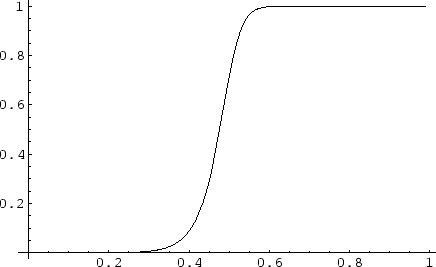
In this case we will see a graph like the one shown in Figure (1.1). The probability of ending up with $21 starting with $15 is very small for probabilities that are less than 1/2. Around 1/2 the chance of success grows very rapidly and if the probability of winning an individual play of the game is larger than 1/2, the chance of success is close to 1.

Figure 1.1: A graph of the chance of success of a gambler as a function of the probability of winning an individual play of the game increases. This is a graph for the case when the gambler starts with $15 and wants to leave with $21.

It is important to note that this simple problem requires a fairly messy solution process. If the problem becomes any more complicated there is no guarantee that we would be able to get an exact representation of the probability. Another point of interest is that the solution process is basically one that we have seen before in an ordinary differential equations course. So we have determined an exact solution for a problem that is a simplification of the problems we first discussed. In general, we will not be able to find exact solutions to the problems that we are faced with. Even the simple examples in the introduction will not lend themselves to the simple analysis we have done. So, we will introduce the concept of doing a simulation of the process. In cases where we cannot determine an exact solution we may be able to get accurate approximate results using a simulation.